Different forms of energy balance equation
The energy balance equation is more complicated, in appearance at least, than the mass balance equation. As one navigates the field of thermofluids, one comes across this equation in several forms. In this article, I want to show you the derivations of these different forms, arriving ultimately to forms that can be implemented into computer code.
To start with, the differential form of the energy balance equation is as follows:
\[\frac {\partial(\rho u V)} {\partial t} = \Sigma \dot mh\]With this equation, we will play around quite a bit. Note that, for simplicity, I didn't add any heat source or transfer terms \(\dot Q\) on the right hand side, but these could be added as needed. For instance, you might have heat transfer to a wall like \(Q = \alpha A(T_{wall}-T_{ref})\). Note also that, for this post, I will write only about rigid control volumes, i.e. the shape doesn't deform, because there is plenty to discuss just within that constraint.
We will also use the following two things:
The mass balance equation \(\frac {\partial(\rho V)} {\partial t} = \Sigma \dot m\)
The fact that enthalpy, \(h = u + Pv\)
First form
First, let me just state that "first form" isn't an official term. It is just that I'm writing this form up first. To start with, we write the enthalpy definition as \(u=h-p/\rho\). This is the same as the second bullet point above, because the volume in that equation is the specific volume, aka the reciprocal of density.
Now, on substituting this into Equation (1) we get:
\[\frac{\partial(\rho(h-P/\rho)V)}{\partial t} = \Sigma\dot mh\] \[\frac{\partial((\rho h-P)V)}{\partial t} = \Sigma\dot mh\] \[V\left(\frac{\partial(\rho h)}{\partial t} - \frac{dP}{dt}\right)= \Sigma\dot mh\]We take volume out of the derivative because it doesn't change with time (and so it's rate of change with time would be zero). Also, we replace the partial derivative \(\partial\) with the derivative \(d\) for pressure. This is because pressure and specific enthalpy are our state variables, aka our independent parameters. Thus, they are functions only of time and not of other thermodynamic parameters.
Two things now. First, we use the product rule[1] on the \(\rho h\) derivative term. Second, we remember that, in thermodynamics, if we know two independent properties, we can determine all other parameters in terms of them. In effect, that is, every property can be expressed as a function of the two independent properties. So, for our purposes, we use this to write \(\rho = f(P,h)\). So that:
\[\frac {\partial \rho}{\partial t} = \frac {\partial \rho}{\partial P} \frac {dP}{dt}\Bigg|_h\ + \frac {\partial \rho}{\partial h} \frac {dh}{dt}\Bigg|_P\ \]Where, the derivatives \(\frac{dP}{dt}\) and \(\frac{dh}{dt}\) are calculated holding the other property constant.
Then, we can do the following with the first derivative term:
\[\frac {\partial(\rho h)} {\partial t} = h\frac {\partial \rho}{\partial t} + \rho\frac {dh}{dt} = h\left(\frac {\partial \rho}{\partial P} \frac {dP}{dt} + \frac {\partial \rho}{\partial h} \frac {dh}{dt}\right)+\rho\frac {dh}{dt}\]Substituting this final term into Equation (4) we get
\[V\left(h\left(\frac {\partial \rho}{\partial P} \frac {dP}{dt} + \frac {\partial \rho}{\partial h} \frac {dh}{dt}\right)+\rho\frac {dh}{dt} - \frac{dP}{dt}\right)= \Sigma\dot mh\]Taking the derivatives common, then:
\[V\left(\left(h\frac {\partial \rho}{\partial P}-1\right) \frac {dP}{dt} + \left(h\frac {\partial \rho}{\partial P}+\rho\right) \frac {dh}{dt} \right) = \Sigma\dot mh\]This form is perhaps familiar to you, since it shows up in many places.
Second Form
Now, let's go back to our original form and add a different flavour to the derivation. First, instead of substituting for \(u\) right away, we instead do the following:
\[u\frac{\partial(\rho V)}{\partial t} + \rho V\frac{\partial u}{\partial t} = \Sigma \dot mh_{bdry}\]That is, we use the product rule [1] to split it into a \(\rho V\) part and a \(u\) part. Note the \(bdry\) subscript I added to the last term this time. This is to emphasise that the enthalpies in the boundary terms may not be the same as the enthalpy of the control volume. Instead, the enthalpies here will be the upstream enthalpy.
Now, maybe you see the next step already, but the first differential term on the left hand side is also the LHS of the mass balance equation \(\frac{\partial(\rho V)}{\partial t}\). We can substitute that in:
\[u \Sigma\dot m + \rho V\frac{\partial u}{\partial t} = \Sigma \dot mh\]And now can add our term for internal energy in terms of enthalpy:
\[\left(h-P/\rho\right)\Sigma\dot m + \rho V \frac{\partial (h-Pv)}{\partial t} = \Sigma\dot mh_{bdry}\]Then, we move some stuff around to get:
\[\rho V \frac{\partial (h-P/\rho)}{\partial t} = \Sigma\dot m\left(h_{bdry}-h+P/\rho\right)\]Now let's simplify the left hand side differential term. We will use the quotient rule[2] here.
\[\rho V\left(\frac{\partial (h-P/\rho)}{\partial t}\right) = \rho V\left(\frac{dh}{dt} - \frac{\partial (P/\rho)}{\partial t} \right) = \rho V\left(\frac{dh}{dt} - \left(\frac{\rho\frac{dP}{dt} -P\frac{\partial\rho}{\partial t}}{\rho^2}\right)\right) = V\left(\rho\frac{dh}{dt}-\frac{dP}{dt}+\frac{P}{\rho}\frac{\partial\rho}{\partial t}\right)\]Ok, things start to look a bit more manageable. The final thing to do is to substitute the terms for the partial derivative of density in terms of pressure and enthalpy, as in the equation above.
\[\frac{P}{\rho}\frac{\partial\rho}{\partial t} = \frac{P}{\rho}\left(\frac {\partial \rho}{\partial P} \frac {dP}{dt} + \frac {\partial \rho}{\partial h} \frac {dh}{dt}\right)\]I got rid of the 'constant pressure/enthalpy' symbols for simplicity.
OK. So the full energy balance equation is:
\[ V\left(\left(\frac{P}{\rho}\frac{\partial\rho}{\partial h}+\rho\right)\frac{dh}{dt} + \left(\frac{P}{\rho}\frac{\partial\rho}{\partial P}-1\right)\frac{dP}{dt}\right) = \Sigma\dot m\left(h_{bdry}-h+P/\rho\right)\]Done.
This form looks considerably more complicated than the previous one, but the equations are the same. It's just a different way to derive. Now, remember that \(h_{bdry}\) is derived from the upwind scheme. This means that, for any flow going OUT of the control volume under consideration, \(h_{bdry} = h\). Then, these terms will cancel out, leaving only \(\dot m_{out}\frac{P}{\rho}\) for all outlet flows.
Another thing to note is that all these \(P/\rho\) stuff only applies to the "flow" things. The source terms \(Q\) are left alone.
Third Form
This one's slightly different.
So far, we've been considering the energy of the control volumes as \(\rho u V\). But this is just a fancy way of saying \(U\), because ultimately, that is what the energy balance equation deals with: that the total energy of the control volume.
In most cases, we can assume that the density \(\rho\) is constant within the control volume, and thus the bulk \(\rho uV = U\) can be taken without issue.
Then, the energy balance equation is written as:
\[\frac{\partial U}{\partial t} = \Sigma\dot mh_{bdry}\]Now, \(U = H - PV\). Here, we are talking extensive properties rather than specific properties (aka per unit mass). The Volume, therefore, is not specific volume, but rather, the volume of the control volume. If we stick this into our equation:
\[\frac{dH}{dt}-\frac{\partial (PV)}{\partial t} = \Sigma\dot mh \]But, Volume doesn't change with time for a rigid control volume. Therefore:
\[\frac{dH}{dt}-V\frac{dP}{dt} = \Sigma\dot mh_{bdry}\]Now, \(H = M*h\). Substituting this and using the product rule:
\[M\frac{dh}{dt} h\frac{dM}{dt} - V\frac{dP}{dt} = \Sigma\dot mh_{bdry}\]And, \(M = \rho V\). So that
\[\rho V\frac{dh}{dt}-h\frac{dM}{dt}-V\frac{dP}{dt} = \Sigma\dot mh_{bdry}\]Finally, \(dM/dt = \Sigma\dot m\) is the mass balance equation. So, if we substitute it in and transport that term to the right hand side, we get
\[\rho V\frac{dh}{dt}-V\frac{dP}{dt} = \Sigma\dot m(h_{bdry}-h)\]Nice. This form is especially enjoyable because of it's simplicity. No partial derivatives are necessary, and the format of the equation is very simple. Note, however, that no partial derivatives are necessary for the energy balance equation. You will still need them for the mass balance calculations.
Implementation
Now, let's implement them into Matlab and do some verifications shall we? I will take the same example I took last time of equal mass flow rate into and out of the control volume. Then, the problem becomes isochoric (constant density) because the total mass inside the control volume never changes.
I will call these forms F1, F2 and F3 respectively. I've talked about the code for F1, I'll skip the code for F2 (and you can take my word for it). Instead, only the F3 code is given below:
function y = controlVolumeF3(~,x)
% controlVolumeF3: Third form of control volume.
% Simplified form described by Richter (2008) and Pini (2013)
% DOES NOT SUPPORT REVERSE-FLOW YET

global fld Vol mDotIn hin mDotOut Qh Qc

P = x(1);
h = x(2);

[drhodPh,drhodhP] = getPartialDers(P,h,fld);
rho = refpropm('D','P',P*1e-3,'H',h,fld);

M = [Vol*drhodPh, Vol*drhodhP;...
	-Vol, rho*Vol];
f = [mDotIn-mDotOut ; mDotIn*(hin-h) + Qh - Qc];

y = M\f;
end
getPartialDers is a function I wrote to calculate the partial derivatives properly in every region, including the two-phase region. It's a (very interesting) topic for another day. The comment screaming that reverse flow isn't supported is saying that here, flow comes in from the inlet port and goes out from the outlet port. There is no possibility of flow coming in from the outlet port. This would require a more rigorous upwind scheme implementation, which I'm too lazy to do.
The comparison between the forms is given below:
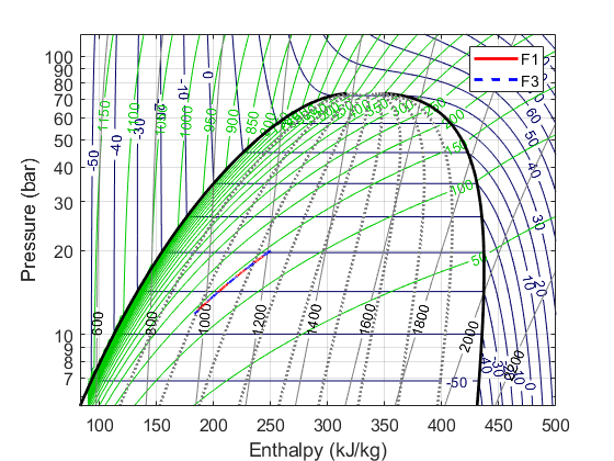
Thus, the results stay the same. Hardly a surprise, of course, considering all we've done is manipulated the maths around without changing the underlying assumption about the physics. But yeah, we've now got some horses for courses.
To be honest, it's hard for me to say why we implement these different forms. I guess it's just an artefact of history that different people derived it different ways when they were dealing with the maths. So far as I can tell, you are free to use either form without hindrance.
| [1] | Product rule: if \(f(x) = u(x).v(x)\), then \(f'(x) = u'(x).v(x)+u(x)v'(x)\) |
| [2] | Quotient rule: if \(f(x) = u(x)/v(x)\), then \(f'(x) = \frac{u'(x)v(x)-u(x)v'(x)}{v(x)^2}\) |