Modelling a control volume in Matlab

Let's discuss how to develop a Minimum Viable Model of a control volume in Matlab. A "control volume" is nothing more than a region of space through which we want to study the flow of a fluid. This is a good exercise because it covers several areas of thermofluids: the upwind scheme, ODEs, calculations of partial derivatives and so on.

Our control volume will represent a pipe: rigid (volume doesn't change) and has two ports (inlet and outlet). We will assume that the wall is perfectly adiabatic, that is, no heat exchange occurs between the pipe and the surroundings bar at the inlet and outlet ports.

Note that if you want to follow along, you will need to have a copy of Matlab (or maybe Octave will do) and the NIST software Refprop (REFrigerant PROPerties).

Preliminaries

Ok, so where do we begin? Well to fully know a control volume, we need to know three things about it: two independent thermodynamic variables and a flow variable. The thermodynamic variables let us calculate all of the properties like density, entropy, vapour quality etc. The flow variable lets us calculate the momentum of the fluid.

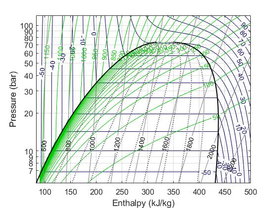
In the field of thermofluids, we often use Pressure and Specific Enthalpy as the state variables. We rely on the pressure-specific enthalpy diagram often to try to make sense of thermodynamic cycles, so it's a natural choice. Also, in the two-phase region (the 'dome' in the P-h diagram below) knowing the enthalpy tells us how far along we are into the two-phase, aka, how much of the fluid we have evaporated/condenesed. This is needed for us in detector cooling applications to know the vapour quality.

Mass flow rate (kg/s) is selected as the flow variable rather than the volumetric flow rate (L/s) or velocity (m/s) because it is more 'objective'. It is unaffected by changes in cross sectional areas. For steady flow, the mass flow rate will be the same everywhere, in a way that the volumetric flow rate and velocity won't be.

We won't do any discretisation of the pipe that we're modelling. In reality, you could subdivide the pipe into smaller segments for more accurate values, but we'll just think of it as one big lump.

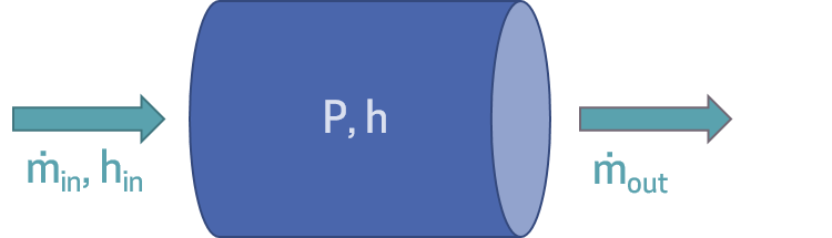
So, we have a 'lumped' volume, and we need to know three things about it: the pressure, the specific enthalpy and the mass flow rate.

Upwind scheme

Let's talk about one of my most favourite mathematical techniques ever. We use the upwind technique to be able to cohesively determine what part of the model calculates what. For the current model, we need the technique to determine what are the boundary conditions, vs what is calculated by the model itself.

We could, if we wanted, solve all three equations inside the same control volume. The trouble is this: the three governing equations all are deeply interconnected. Changes in one equation will have impacts on the other equations. We call this having the equations 'coupled'. This is a nightmare situation for the differential equation solvers because it brings them to a crawl.

To avoid this, Courant et al^[1], back in 1952, proposed the upwind scheme, which was later covered by Patankar^[2] in his brilliant 1980 book. Using this method, we 'decouple' the equations from each other. We solve the mass and energy balance on one grid called the 'thermal grid', and, offset by half a cell width, we solve the momentum balance on the 'momentum grid'.

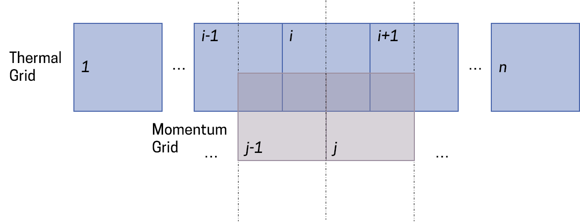
The cells are the same width, and thus, offsetting by half a cell-width means that the centers of one grid coincide with the boundaries of the other grid. This way, whatever is calculated inside one grid is automatically averaged right at the boundary of the neighbouring grid, and thus no interpolation is necessary.

This concept is pretty tricky to understand, but ultimately, it's sufficient if you remember that, if we're dealing with a capacitive component, the mass flow rate is determined by the upwind scheme, and, if we're dealing with a resistive component, the pressure is determined by the upwind component. The incoming enthalpy, meanwhile, is ALWAYS determined by upstream conditions.

Boundary and Initial Conditions

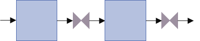
So, having discussed the upwind scheme, we now take the control volume itself to be a 'capacitive' element. That is, the control volume solves for the pressure and specific enthalpy using the mass and energy balance equations. Then, the inlet and outlet ports must supply the 'resistive' element of the equation, aka the mass flow rate. Then, just before the inlet port would be some momentum grid element, and likewise for just beyond the outlet port, were we to build up a complete system model.

Note, however, that in addition to the mass flow rate, we also need to supply the enthalpy of the incoming fluid, as the upwind scheme dictates that the inlet enthalpy be defined by the component upstream of it. Thus, the system setup ends up looking like:

In addition, when solving differential equations that involve time, we need to provide initial conditions. We need as many initial conditions as there are dynamic variables, two in this case (pressure and enthalpy).

The equations

Now, let's talk about the governing equations. First, the mass balance.

Mass Balance

Our flow is one-dimensional. Thus, our equation will take the form:

\[\frac{\partial{(\rho V)}}{\partial t} = \dot{m}_{in}-\dot{m}_{out}\]

Rather straightforward, right? The equation basically states that any refrigerant flowing into the control volume can do one of two things: 1) increase the mass inside the volume, or 2) flow out of the volume.

Notice, however, that our volume is not deformable. The control volume is rigid, and thus the derivative of Volume with time will be zero. The equation then becomes:

\[V\frac{\partial{(\rho)}}{\partial t} = \dot{m}_{in}-\dot{m}_{out}\]

Next, we notice that the equation above is in terms of density, and not in terms of pressure and specific enthalpy, which are our state variables. So what do we do?

We first remember that in thermodynamics, any variable can be found using two other known variables. Then, \(\rho=f(P,h)\)

If we apply the chain rule of differentiation to this fact, we get

\[V\frac{\partial{\rho}}{\partial t} = \frac{\partial\rho}{\partial P}\frac{dP}{dt}\Bigg|_h + \frac{\partial\rho}{\partial h}\frac{dh}{dt}\Bigg|_P\]

Here, the pipe symbols with the subscripts mean that when we are taking the partial derivative of the pressure, we keep enthalpy constant (and vice versa).

Substituting this into the mass balance equation gives:

\[V\left(\frac{\partial\rho}{\partial P}\frac{dP}{dt}\Bigg|_h + \frac{\partial\rho}{\partial h}\frac{dh}{dt}\Bigg|_P\right) = \dot{m}_{in}-\dot{m}_{out}\]

These partial derivatives will be calculated using Refprop and some fluid property magic in the two-phase region. But now let's do the same for the energy balance.

Energy Balance

The energy balance equation will look like this:

\[\frac{\partial{(\rho uV)}}{\partial t} = \dot{m}h_{in}-\dot{m}h_{out}\]

This equation is along the same lines as the previous ones, stating that if we have a flow coming in (carrying energy), it can either flow out, or raise the internal energy of the fluid inside.

Now, as before, we note that the volume is constant. So, we are left with \(\rho.u\) inside the derivative. Then, we also know that the enthalpy is \(h = u + P/\rho\). Thus, \(u = h - P/\rho\). If we substitute this into the equation above and run the crank of deriving it out, we will get:

\[V\left(\left(h\frac{\partial\rho}{\partial P}-1\right)\frac{dP}{dt}\Bigg|_h + \left(h\frac{\partial\rho}{\partial h}+\rho\right)\frac{dh}{dt}\Bigg|_P\right) = \dot{m}h_{in}-\dot{m}h_{out}\]

Implementing the code in Matlab

Right! Onto the good stuff. How do we implement this in matlab? Let's first try to understand how ODEs are set up in Matlab. Well, ODEs are set up in the form of matrix equations in Matlab. They take the form Ax = B, with x being the vector of state variables, A is the matrix of the partial derivatives, while B contains the constraints, or the boundary conditions in our example.

\[ \left[ \begin{matrix} V\frac{\partial\rho}{\partial P} & V\frac{\partial\rho}{\partial P} \\ V\left( h\frac{\partial\rho}{\partial P} - 1\right) & V\left(h\frac{\partial\rho}{\partial P} +\rho \right) \end{matrix} \right] \left[\begin{matrix}{\partial P}/{\partial t} \\ {\partial h}/{\partial t}\end{matrix}\right] = \left[ \frac{\dot{m}_{in}-\dot{m}_{out}}{\dot{m}h_{in}-\dot{m}h_{out}}\right] \]

Then, if we are able to set up a function that returns the values of these partial derivatives, we can send this to our ODE function, and it can integrate the equation over time. Thus, we need a function that outputs x = A\B

Let's look at that code now.

function y = controlVolume(~,x,fld,Vol,mDotIn,hin,mDotOut)
% controlVolume Lumped control volume
% Inlet boundary conditions: mass flow rate and enthalpy
% Outlet boundary condns: mDot
% State variables: Pressure (Pa) and enthalpy (J/kg)

P = x(1); % Pa
h = x(2); % J/kg

% Function I wrote to calculate two-phase partial derivatives:
[drho_dPh,drho_dhP] = getPartialDers(P,h,fld); 

rho = refpropm('D','P',P*1e-3,'H',h,fld);

Hin = mDotIn*hin;
Hout = mDotOut*h;

a = Vol*drho_dPh;
b = Vol*drho_dhP;    
c = Vol*(h*drho_dPh-1);
d = Vol*(h*drho_dhP+rho);

M = [a,b ; c,d];
f = [mDotIn-mDotOut ; Hin-Hout];

y = M\f;
end

This code should hopefully look pretty understandable to you by now. The matrices A and B are here called M and f to be more consistent with the implicit equation nomenclature that Matlab uses. Don't worry about it. It's just another name.

So, what is this function spitting out? The values of dy/dt, aka [dP/dt ; dh/dt]. The getPartialDerivatives function calculates the partial derivatives, mindful of where we are in the Pressure-enthalpy diagram (single phase or two-phase).

% LUMPED CONTROL VOLUME - P/h STATE VARIABLES
% Pressure (Pa) and specific enthalpy (J/kg) state variables
% Inlet and outlet mass flow rates and enthalpies boundary conditions
% (Note: Pressure in Pa for state var, bar for plots and kPa for refprop)

clc
clear
close all

fld = 'CO2';

% Time discretization
t = 60; % Simulation time [s]
dt = 1; % [s]
tspan = 0:dt:t;
nt = length(tspan);

% Geometry
D = 0.2; % [m]
L = 0.32; % [m]
Vol = pi * (D/2)^2 * L; % [m3]

% Boundary Conditions
mDotIn = 0.01; % [kg/s]
hin = 100000; % [J/kg]
mDotOut = 0.01;

% Initial Conditions
P0 = 20e5; % Pa
h0 = 250000; % J/kg
x0 = [P0,h0]; %

% Solving ODEs
optionSet = odeset('OutputFcn',@odeplot,'RelTol',1e-5);
[t,x] = ode15s(@(t,x) controlVolume(t,x,fld,Vol,mDotIn,hin,mDotOut), tspan, x0, optionSet);

% Plotting
set(0,'defaultlinelinewidth',1.5);
set(0,'DefaulttextFontSize',14);
set(0,'DefaultaxesFontSize',10);
P = x(:,1).*1e-5;
h = x(:,2).*1e-3;
plotPh(); % my own function for plotting the pressure-enthalpy diagram
plot(h,P,'r');
text(h(1),P(1),'\leftarrow Start');
text(h(end),P(end),'\leftarrow End');

Right, so a couple of things to comment here. First the simulation parameters. The way I set up the simulation above is to have a 10 L vessel, full of a two-phase mixture of CO2. Then, we have 10 g/s flowing in, and 10 g/s flowing right out again. The incoming fluid is at very cold enthalpies of 100 kJ/kg (corresponding to < -45°C at 20 bar).

So, what would you expect? Well, since the flow rate in and flow out is the same, the mass should stay constant. And indeed, that is what we see. Look at the P-h diagram below

The green lines are the isochores, aka the constant density lines. The red line, as you can see, proceeds along the constant density line. Slowly, the control volume is also cooling down. All seems to make sense.

So, what have we achieved? Well, if you were able to follow along, you should now be able to create what is the basic component for all thermofluid simulations. By creating successions of such control volumes, we can model very complex systems indeed, and that is something I hope to continue talking about in future posts.

References

[1]	Courant, R., Isaacson, E., & Rees, M. (1952). On the solution of nonlinear hyperbolic differential equations by finite differences. Communications in Applied Numerical Methods, 5(3), 243–255. http://doi.org/10.1002/cpa.3160050303

[2]	Patankar, S. (1980). Numerical heat transfer and fluid flow. Series in Coputational Methods in Mechanics and Thermal Sciences. http://doi.org/10.1016/j.watres.2009.11.010